How to check if a time series data is stationary
A stationary time series is a series whose statistical properties such as mean, variance, and autocorrelation are constant over time. A stationary series has the same distribution at every point in time, and the distribution does not change over time.
There are two main types of stationarity that are relevant in time series analysis:
-
Strict stationary: A time series is said to be strictly stationary if the joint distribution of any set of observations is invariant to time shifts. That is, the distribution of any group of observations remains the same, regardless of the time at which they were observed.
-
Weak stationary: A time series is said to be weakly stationary if the mean, variance, and autocorrelation structure of the series do not change over time. In other words, the mean and variance of the series are constant over time, and the autocorrelation between any two observations only depends on the time lag between them, and not on the absolute time at which they were observed.
To test for stationarity, there are several statistical tests available, including:
-
Visual inspection: A simple way to check for stationarity is to plot the time series and visually inspect it for trends, seasonality, and other patterns that might indicate non-stationarity.
-
Summary statistics: Summary statistics such as the mean, variance, and autocorrelation can also provide clues about the stationarity of a series. If the mean and variance are roughly constant over time, and the autocorrelation decreases quickly to zero as the lag increases, then the series is likely stationary.
-
Augmented Dickey-Fuller (ADF) test: The ADF test is a popular statistical test used to determine whether a series is stationary. The test involves regressing the series on its lagged values and testing for the significance of the coefficient on the lagged value. If the coefficient is not significantly different from zero, then the series is likely stationary.
-
KPSS test: The Kwiatkowski-Phillips-Schmidt-Shin (KPSS) test is another statistical test used to determine the stationarity of a series. The test involves regressing the series on a constant and a time trend, and testing for the significance of the trend coefficient. If the trend coefficient is not significantly different from zero, then the series is likely stationary.
In summary, a stationary time series is one whose statistical properties do not change over time. There are several methods available to test for stationarity, including visual inspection, summary statistics, and statistical tests such as the ADF and KPSS tests.
Methods to handle Non-stationary time series data
Yes, there are several modeling approaches that can be used to deal with non-stationary time series data:
-
Differencing: One of the most common methods to make a time series stationary is to apply differencing. This involves taking the first or second difference of the series to remove the trend or seasonal components. Once differenced, the series may be more amenable to modeling using methods that assume stationary data.
-
Transformation: Another approach is to transform the data using a logarithmic, square root, or power transformation to stabilize the variance of the series.
-
ARIMA models: Autoregressive Integrated Moving Average (ARIMA) models are widely used to model stationary time series. However, ARIMA models can also be used for non-stationary series by first differencing or applying other transformations to make the series stationary.
-
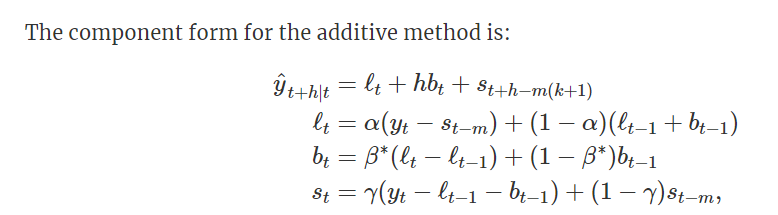
Exponential smoothing models: Exponential smoothing models, such as the Holt-Winters method, are useful for modeling time series data with a trend and/or seasonal component, even if the series is non-stationary.
-
Structural time series models: Structural time series models can handle non-stationary time series by modeling the underlying trend, seasonal, and cyclical components separately, allowing for more flexibility in modeling non-stationary data.
-
Deep learning models: Deep learning models such as recurrent neural networks (RNNs) and long short-term memory (LSTM) networks can handle non-stationary time series by learning the underlying patterns in the data, including trends and seasonal cycles.
In summary, while non-stationary time series data can pose challenges for traditional statistical methods, there are a variety of techniques available to model and analyze this type of data. The choice of method will depend on the specific characteristics of the data and the research question at hand.
A Brief History of Time Series Models
TL;DR: For folks who are interested in learning more about time series models, below is an incomplete roadmap that attempts to summarize the development of this complex, fast evolving field.
M Competition is the equivalence of ImageNet to computer vision for time series model and deep learning beat traditional statistical models for the first time in M4 that took place in 2018 despite all the advancement in computer visions and NLP prior to that. For univariate forecasting, I would recommend trying N-BEATS and N-HiTS while TFT shows good promise for multivariate forecasting. If your time series is too short for deep learning model, you may want to try multi-task (or, is it meta?) learning by using the M4 data as shown in ESRNN. As always, if the simpler approach such as Exponential Smoothing and ARIMA(X) works, it is unnecessary to go nuclear with deep learning. For instance, the Theta model won the M3 competition. Finally, if you can only afford one Python package for time series model, you won’t regret by going with Darts.
Competitions
M Competition is the equivalence of ImageNet to computer vision for time series model. Traditional statistical models had always dominated the competitions until M4 where a hybrid approach of Exponential Smoothing and RNN proposed by Uber called ESRNN won the competition. There are typically several publications after the M competitions that summarize the findings and we can learn a lot from them. M6 is currently ongoing focusing on financial time series. Below is a list of relevant competitions (for M competition, the year refers to the year of publication). Obviously, there are also multiple relevant competitions on Kaggle but they are not included here.
-
1982 — M1
-
1993 — M2
-
2006 — NN3
-
2008 — NN5
-
2021 — M5: LightGBM was the winner on Walmart hierarchical time series sales data (ended in June 2020)
-
2023 — M6: Currently ongoing till the beginning of 2023 on financial time series
Statistical and ML Models
Below is a chronology of both statistical and ML time series models. It is not a comprehensive list but should capture the key development. Also, the timeline is not exact as the year when something was “formally” released or published can sometimes be ambiguous.
-
1950s — Exponential Smoothing
-
1970s — ARIMA(X)
-
1980 — VAR
-
1980s — GARCH
-
2000 — Theta model
-
2011 — TBATS
-
2016 — LightGBM (Microsoft)
-
2017 — CatBoost (Yandex)
-
2017 — Prophet (Facebook)
-
2017 — DeepAR (Amazon)
-
2017 — Multi-Horizon Quantile Recurrent Forecaster — MQRNN (Amazon)
-
2018 — Temporal Graph Convolutional Network — T-GCN (Central South University, Changsha, China)
-
2018 — ESRNN (Uber)
-
2019 — N-BEATS (ElementAI)
-
2019 — AR-Net (Facebook)
-
2020 — NeuralProphet (Facebook)
-
2021 — ThymeBoost
-
2021 — Orbit (Uber)
From Exponential Smoothing in the 1950s and ARIMA(X) in the 1970s to TBATS in 2011, traditional statistical models dominated the time series field especially for univariate forecasting until ESRNN won M4 in 2018. Although NLP essentially works with sequences, a lot of the advancement in NLP cannot be translated to time series effectively because regular time series data lacks the deep structure prevalent with text data. So, in order to make deep learning works for time series, specific neural network architecture is required. N-BEATS is one such example and it outperforms ESRNN for M4 data while N-HiTS subsequently become the state-of-the-art. For NLP fans who are obsessed with attention and transformer, you should be excited about Temporal Fusion Transformer (TFT) proposed by Google in 2020. It works well for multivariate forecasting.
ESRNN introduced a form of multi-task (or, is it meta?) learning that is critical for common business application. Deep learning typically requires a lot of data. While an electricity demand forecasting problem with minute by minute weather data for a large region over the last ten years can easily satisfy the most complex deep neural network, most business applications deal with monthly or quarterly data say for the last ten years (if you are lucky). Instead of building one model (single task) for each time series like a traditional statistical model would do, ESRNN feed all the data into one complex model to forecast multiple time series (multi-task). For example, in M4, there are 24,000 quarterly time series that originated from different domains covering different time period. This is particularly relevant when you have hierarchical data such as different products in the same store or same product across many stores.
N-BEATS introduced another important approach of ensembling models with different input horizons (2x to 7x of forecast horizon), metrics and random initializations for bagging. They found that it is a more helpful regularization technique compared to using dropout or L2 norm penalty.
Gradient boosting algorithms such as XGBoost and LightGBM are not exactly time series models but one can often reduce a time series problem into something more cross-sectional-like. For example, LightGBM won the M5 competition for hierarchical time series. ThymeBoost is a gradient boosting model designed specifically for time series but it is still relatively new. Currently, it does not consistently outperform ESRNN for M4 data.
If you are working with time series that has a heavy seasonal component with strong holiday effect (think Facebook and Linkedin), you may find Prophet and Greykite helpful but they are not based on deep learning. Facebook subsequently adapted AR-Net into Prophet and created NeuralProphet which is essentially a deep learning extension of ARIMA just like how ESRNN is a deep learning extension of Exponential Smoothing.
Packages
Below are some Python packages that are useful for time series forecasting and they implement some of the algorithms mentioned above. Darts is particularly useful for trying multiple advanced algorithms along with helpful functions such as rolling cross validation etc. which are also provided by sktime. AutoML is a relatively new entrant for time series models with PyCaret and some automated feature engineering libraries. Note that one interesting feature engineering method is to apply Fourier transformation on calendar dates (more discussion here).
If you miss the old-school econometrics concepts such as Augmented Dickey Fuller test for stationarity, Breusch-Pagan test for heteroskedasticity and Ljung-Box test for autocorrelation, statsmodels will prove to be handy. “Forecasting: Principles and Practice” is a classic text book for old-school time series models.
-
statsmodels — Standard statistical models such as ARIMA(X), exponential smoothing, Theta, VAR and useful tools such as various statistical tests, acf/pacf plots, time series decomposition etc.
-
pmdarima — Automated ARIMA
-
sktime (2019) — Sklearn-like library for time series with AutoETS and AutoARIMA including utility for rolling cross validation and grid search
-
PyTorch Forecasting (2020) — State-of-the-art time series forecasting with deep neural networks
-
Darts (2020) — A hybrid of sktime and PyTorch Forecasting
-
PyCaret (2021) — AutoML for time series recently integrated into the stable release
-
tsfresh and tsfeatures — Automated feature engineering for time series
Appendix
Here is a quick summary for a few selected models mentioned above. It is impossible to do justice to them with the short descriptions below. So, I would recommend that you do more research to further your understanding.
Exponential Smoothing
One naive forecast approach is to simply use the last observed value as the next prediction. One could also take the simple average of all observed data to make the forecast. Exponential smoothing is in between these two extreme approaches giving larger weights to more recent observations.

This simple concept was subsequently extended to have an error/level, trend and seasonal component with either additive or multiplicative formulation.
“Forecasting: Principles and Practice”, Hyndman et al. (2021)
ARIMA(X)
An autoregressive model uses the lagged values of the target as predictors in a regression. An autoregressive model of order p can be written as:

Rather than using the past values of the forecast variable in a regression, a moving average model uses past forecast errors in a regression-like model.

These two approaches can be combined into one framework which was subsequently extended to capture seasonality and additional regressors. Note that the time series has to be stationary to satisfy the underlying assumptions of the model. Typically taking the first difference of the time series would render it stationary.
Theta Model
The original Theta method proposes the decomposition of the de-seasonalized data into two theta lines. The first theta line removes completely the curvature of the data, thus being a good estimator of the long term trend component. The second theta line doubles the curvature of the series, as to better approximate the short-term behavior. A generalization of the Theta method was subsequently proposed to optimize the selection of the second theta line.
TBATS
This model forecasts time series with complex multiple seasonal patterns using exponential smoothing. The acronym stands for:
-
T — Trigonometric seasonality
-
B — Box-Cox transformation
-
A — ARIMA errors
-
T — Trend
-
S — Seasonal components
Prophet
A modular regression model with interpretable parameters that can be intuitively adjusted by analysts with domain knowledge about the time series. The specification is similar to a generalized additive model (GAM) framing the forecasting problem as a curve fitting exercise with interpretable parameters and components. Also, additional regressors can be accommodated. Note that the default behavior is to rely on the first 80% of the data for the trend component when making future forecast. This may or may not make sense for your application.
“Forecasting at Scale”, Taylor et al. (2017)
ESRNN
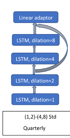
The model cleverly combines the classic Exponential Smoothing model (ES) and a Recurrent Neural Network (RNN). The ES decomposes the time series in level, trend and seasonality components. The RNN is trained with all the series, has shared parameters and it is used to learn common local trends among the series while the ES parameters are specific for each time series. The models are combined by including the output of the RNN as the local trend component in the ES model. Note that the basic architecture is a dilated-RNN with LSTM cells, this allowed the RNN to reduce the number of parameters while stacking more layers.
The ESRNN model optimizes over two losses. First, the quantile loss which minimize the quantile of the target variable and second, a penalty on the variance or wiggliness of the predictions as a regularizer. Intuitively, the level should be a smooth version of the time series, with no seasonality patterns. It turned out that the smoothness of level helped substantially the forecasting accuracy. It appears that when the input to the NN was smooth, the NN concentrated on predicting the trend, instead of overfitting on some spurious, seasonality-related patterns. A smooth level also means that the seasonality components properly absorbed the seasonality.
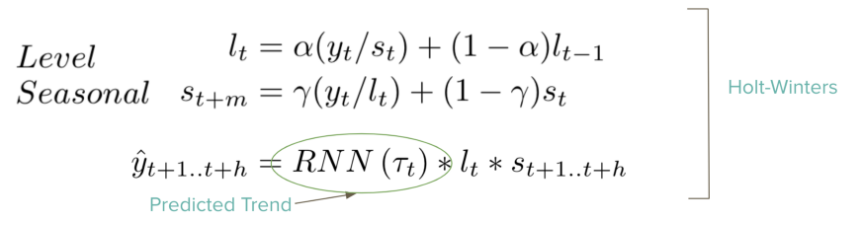
“A hybrid method of Exponential Smoothing and Recurrent Neural Networks for time series forecasting”, Smyl (2019)
N-BEATS
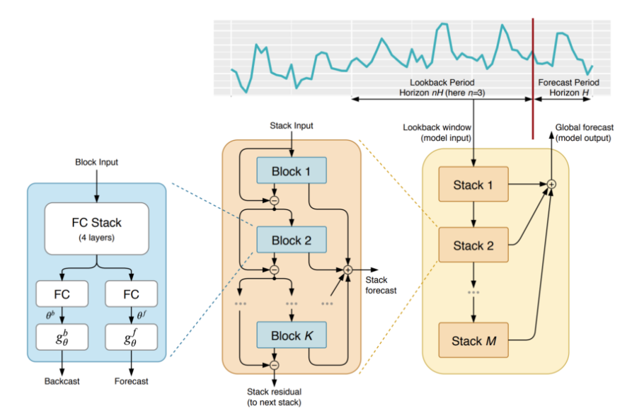
This is the first work to empirically demonstrate that pure DL using no time-series specific components outperforms well-established statistical approaches on M3, M4 and TOURISM datasets. It focuses “on solving the univariate time series point forecasting problem using deep learning”. Subsequently, the Darts package adapts the original N-BEATS architecture to multivariate time series by flattening the source data to a 1-dimensional series. So, you can include additional regressors as features.
Note that N-BEATS is not based on a recurrent architecture such as LSTM. N-BEATS uses a simple but powerful architecture of ensembled feed-forward networks with a novel hierarchical doubly residual topology of forecasts and ‘backcasts’. Previous block removes the portion of the signal that it can approximate well, making the forecast job of the downstream blocks easier. The proposed architecture design generalizes well across time series of different nature while ESRNN had to use very different architectures hand crafted for different horizons. Finally, if interpretability is important for your application, this model offers an “interpretable” architecture consisting of two stacks: A trend stack and a seasonality stack.
“N-BEATS: Neural basis expansion analysis for interpretable time series forecasting” , Oreshkin et al. (2020)
Temporal Fusion Transformer (TFT)
TFT is an attention-based DNN designed to explicitly align the model with the general multi-horizon forecasting task, i.e. predicting variables-of-interest at multiple future time steps, for both accuracy and interpretability. TFT supports 3 types of features: i) temporal data with known inputs into the future ii) temporal data known only up to the present and iii) exogenous categorical/static variables. See more discussion here.
The architecture integrates the mechanisms of several other neural architectures:
-
A temporal multi-head attention block that identifies the long-range patterns
-
LSTM sequence-to-sequence encoders/decoders to summarize shorter patterns
-
Gated residual network blocks, GRNs, that are to weed out the unimportant, unused inputs

“Temporal Fusion Transformers for Interpretable Multi-horizon Time Series Forecasting”, Lim et al. (2020)
This article represents my own opinion and does not necessarily represent the opinions of T. Rowe Price, and has not been sanctioned by T. Rowe Price.