Stock Prediction with LorenzANN
Introduction

LorenzANN, the algorithm of Approximate Nearest Neighbors Search with Lorentzian Distance, has gained popularity as a customized machine learning tool. Some youtubers even consider it to be one of the best machine learning indicators available.
Core Method
The cusomized LorenzANN algorithm uses the following methodology:
-
The algorithm maintains a list of the k-similar neighbors simultaneously in both a predictions array and a corresponding distances array.
-
If the predictions array size exceeds the number of nearest neighbors specified in settings.neighborsCount, the algorithm removes the first neighbor from both the predictions array and the corresponding distances array.
-
The lastDistance variable is overridden to be a distance in the lower 25% of the array. This step helps to increase accuracy by ensuring that newly added distance values increase at a slower rate.
-
Lorentzian distance is used as a distance metric, which minimizes the effect of outliers and takes into account the warping of “price-time” due to proximity to significant economic events.
Python Example
While the source code for LorenzANN is shared on TradingView, there are certain limitations to its use. Firstly, the algorithm is hard-coded with fixed inputs and can only handle a maximum of five features. Additionally, it is written in Pine-Script, which embeds the core logic with visualization logics, making it difficult to separate the two functionalities.
To overcome the limitations of the LorenzANN algorithm, I have translated the code shared on TradingView from Pine-Script to Python. The translated code is now capable of handling any number of features, making it more flexible than the original version. This updated algorithm has been successfully integrated into my trading bot, allowing me to utilize its enhanced capabilities for my trading strategies.
def approximate_nearest_neighbors(df, y_col, x_cols, sampling_factor=4, neighber_count=8, look_back_period=80):
    '''
    1. The algorithm iterates through the dataset (df) in chronological order,
    using the modulo operator to only perform calculations every sampling_factor bars, where sampling_factor= 4.

    2. This serves the dual purpose of reducing the computational overhead of the algorithm
        and ensuring a minimum chronological spacing between the neighbors of at least sampling_factor bars,
        where sampling_factor = 4.

    3. A list of the k-similar neighbors is simultaneously maintained in both
    a predictions array and corresponding distances array.
    When the size of the predictions array exceeds the desired number of nearest
    neighbors specified in neighber_count, where neighber_count=8,
    the algorithm removes the first neighbor from the predictions array
    and the corresponding distance array.

    4. The lastDistance variable is overriden to be a distance in the lower 25% of the array.
    This step helps to boost overall accuracy by ensuring subsequent newly added distance values increase at a slower rate.
    '''
    assert len(df)> look_back_period

    res = [None]* look_back_period
    for i in tqdm(range(look_back_period, len(df))):
        row = df.iloc[i]
        predictions = []
        distances = []
        last_dist = -1
        for pre_i in range(i-look_back_period, i):
            # sampling
            if pre_i % sampling_factor == 0:
                pre_row = df.iloc[pre_i]
                # Calculate Lorentzian distance and add to distances array
                distance = lorentzian_distance(row[x_cols].values, pre_row[x_cols].values)
                if distance > last_dist:
                    distances.append(distance)
                    # Add prediction to predictions array
                    predictions.append(np.round(df[y_col].iloc[i]))

                # If number of neighbors is greater than neighber_count, remove the first neighbor
                if len(predictions) > neighber_count:
                    predictions = predictions[1:]
                    distances = distances[1:]

                # Override last_dist to be a distance in the lower 25% of the array
                # this is like the time-decay factor
                if distances:
                    last_dist = np.percentile(distances, 25)
        res.append(np.mean(predictions))
    return res
Notice that the result will be different on TradingView since the overall shared trading stratgy also including some technical filters like golden cross with 200 EMA/SME … etc.
Summary
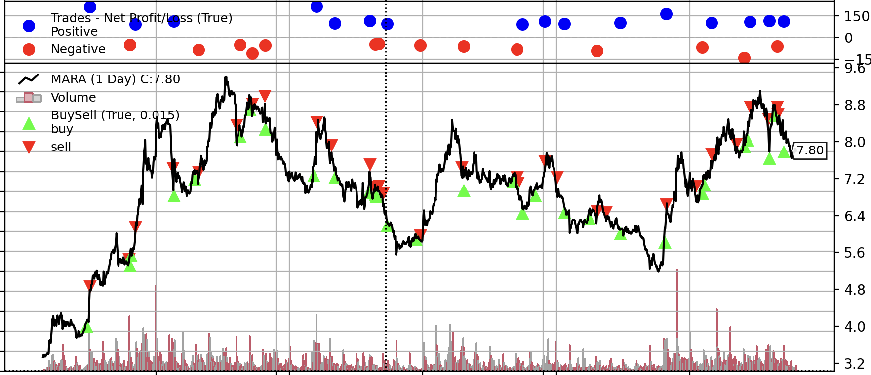
Overall, the method with some technical indicators as input did show some profitable experiment during the backtesting. For example as below backtesting reuslt.
Simulation Result
Key Statistic
| Item | Value |
|---|---|
| Back Test Start | 2023-01-03 |
| Back Test End | 2023-03-24 |
| Back Test Cash | 29000 |
| Frequency | 15 min |
| Sharp-Ratio | 1.7 |
| max_drawdown | 3102 |
| return_value | 9042 |
| return_to_mdd_ration | 2.91 |
| return_per_day | 113 |